Deep Learning: A Comprehensive Guide

Deep Learning, a subfield of machine learning, has revolutionized numerous domains, from image recognition and natural language processing to robotics and medical diagnosis. Its power lies in its ability to learn intricate patterns from vast amounts of data through artificial neural networks with multiple layers. This blog post will delve into the fundamental concepts of deep learning, explore its key components, and provide a technical understanding of its inner workings.

The Foundation: Neural Networks

At the heart of deep learning lies the artificial neural network (ANN), inspired by the structure and function of the human brain. A basic neural network consists of interconnected nodes or "neurons" organized in layers:

• 
• Input Layer: Receives the raw data.
• Hidden Layers: Perform the computations and feature extraction. Deep learning models are characterized by having multiple hidden layers.
• Output Layer: Produces the final prediction or classification.

Each connection between neurons has an associated weight, which determines the strength of the connection. Neurons also have a bias, which acts as an offset. When a neuron receives signals from the neurons in the preceding layer, it calculates a weighted sum of these inputs, adds the bias, and then applies an activation function.

Activation Functions: Introducing Non-Linearity

Activation functions are crucial as they introduce non-linearity into the network. Without them, a deep neural network would essentially behave like a single linear layer, severely limiting its ability to learn complex relationships. Some common activation functions include:

• Sigmoid: Outputs a value between 0 and 1, often used in binary classification problems.
• Tanh (Hyperbolic Tangent): Outputs a value between -1 and 1.
• ReLU (Rectified Linear Unit): Outputs the input if it's positive, and 0 otherwise (f(x) = max(0, x)). ReLU is widely used due to its simplicity and effectiveness in avoiding the vanishing gradient problem (discussed later).
• Leaky ReLU: A variation of ReLU that allows a small, non-zero gradient when the input is negative, addressing the "dying ReLU" problem.
• Softmax: Used in the output layer for multi-class classification, it converts a vector of raw scores into a probability distribution over the classes.

The "Deep" in Deep Learning: Multi-Layer Architectures

The defining characteristic of deep learning is the presence of multiple hidden layers. These layers enable the network to learn hierarchical representations of the data. For instance, in image recognition:

• The initial layers might learn to detect edges and corners.
• Subsequent layers could combine these features to identify shapes and textures.
• Deeper layers could then assemble these into higher-level objects like eyes, noses, or wheels.

This hierarchical feature learning is what allows deep learning models to excel in tasks where the underlying patterns are complex and abstract.

Learning the Weights: The Role of Loss Functions and Optimization

The process of training a deep learning model involves adjusting the weights and biases to minimize the difference between the network's predictions and the actual target values. This difference is quantified by a loss function (also called a cost function or objective function). Common loss functions include:

• Mean Squared Error (MSE): Used for regression tasks, it calculates the average squared difference between the predicted and true values.
• Binary Cross-Entropy: Used for binary classification, it measures the dissimilarity between the predicted probabilities and the true binary labels.
• Categorical Cross-Entropy: Used for multi-class classification, it extends binary cross-entropy to more than two classes.

Once the loss function is defined, an optimization algorithm is used to iteratively update the weights and biases in the direction that reduces the loss. The most fundamental optimization algorithm is Gradient Descent.

Gradient Descent: Navigating the Loss Landscape

Gradient descent works by calculating the gradient of the loss function with respect to the network's parameters (weights and biases). The gradient indicates the direction of the steepest increase in the loss. Therefore, to minimize the loss, the parameters are updated in the opposite direction of the gradient:

θ = θ - α ∇J(θ)

Where:

• θ represents the network's parameters (weights and biases).
• α is the learning rate, a hyperparameter that controls the step size during optimization.
• ∇J(θ) is the gradient of the loss function J with respect to θ.

Several variations of gradient descent are used in practice:

• Batch Gradient Descent: Calculates the gradient based on the entire training dataset. While providing an accurate gradient, it can be computationally expensive for large datasets.
• Stochastic Gradient Descent (SGD): Updates the parameters based on the gradient calculated for a single randomly chosen training example. This is much faster per iteration but can have noisy updates.
• Mini-Batch Gradient Descent: Calculates the gradient on a small random subset (mini-batch) of the training data. This offers a compromise between the efficiency of SGD and the stability of batch gradient descent.

Advanced Optimization Algorithms

Beyond basic gradient descent, various advanced optimization algorithms have been developed to improve training speed and stability. Some popular ones include:

• Momentum: Adds a fraction of the previous update vector to the current update, helping to accelerate convergence and overcome local minima.
• RMSprop (Root Mean Square Propagation): Adapts the learning rate for each parameter based on the magnitudes of recent gradients.
• Adam (Adaptive Moment Estimation): Combines the ideas of momentum and RMSprop, often providing good performance across a wide range of tasks.

Backpropagation: The Engine of Learning

The efficient computation of gradients for all the parameters in a deep neural network is made possible by the backpropagation algorithm. It utilizes the chain rule of calculus to propagate the error (the difference between the predicted and actual output) backward through the network, layer by layer.

Here's a simplified overview of the backpropagation process:

1. Forward Pass: Input data is fed through the network, and the output is calculated for each layer.
2. Error Calculation: The loss function is computed based on the network's output and the true target values.
3. Backward Pass: The gradient of the loss function with respect to the parameters in the output layer is calculated. This gradient is then propagated backward through the network, calculating the gradient with respect to the parameters in each preceding layer using the chain rule.
4. Parameter Update: The optimization algorithm uses the calculated gradients to update the weights and biases.

This iterative process of forward pass, error calculation, backward pass, and parameter update continues until the network converges to a state where the loss is minimized.

Challenges in Deep Learning

Training deep learning models is not always straightforward and comes with its own set of challenges:

• Vanishing and Exploding Gradients: During backpropagation, gradients can become extremely small (vanishing) or very large (exploding) as they are propagated through many layers. Vanishing gradients can hinder learning in earlier layers, while exploding gradients can lead to unstable training. Techniques like ReLU activation, gradient clipping, and careful weight initialization help mitigate these issues.
• Overfitting: This occurs when a model learns the training data too well, including the noise and random fluctuations, and fails to generalize to unseen data. Techniques to combat overfitting include:
  • Regularization: Adding penalties to the loss function based on the magnitude of the weights (e.g., L1 and L2 regularization).
  • Dropout: Randomly deactivating a fraction of neurons during training, forcing the network to learn redundant representations.
  • Data Augmentation: Creating new training examples by applying transformations (e.g., rotations, flips, crops) to the existing data.
  • Early Stopping: Monitoring the model's performance on a validation set and stopping training when the performance starts to degrade.
• Computational Cost: Training deep learning models often requires significant computational resources (GPUs or TPUs) and time, especially for large datasets and complex architectures.
• Hyperparameter Tuning: Deep learning models have numerous hyperparameters (e.g., learning rate, number of layers, number of neurons per layer, regularization strength, dropout rate) that need to be carefully tuned to achieve optimal performance. This often involves experimentation and techniques like grid search, random search, or more advanced optimization methods.
• Interpretability: Deep learning models, especially very deep ones, can be like "black boxes," making it difficult to understand why they make certain predictions. This lack of interpretability can be a concern in critical applications. Research in explainable AI (XAI) is actively addressing this challenge.

Popular Deep Learning Architectures

Over the years, various deep learning architectures have been developed, each tailored for specific types of data and tasks:

• Convolutional Neural Networks (CNNs): Primarily used for image and video processing. They utilize convolutional layers to automatically learn spatial hierarchies of features.
  • Recurrent Neural Networks (RNNs): Designed for sequential data like text, audio, and time series. They have feedback connections that allow them to maintain a "memory" of past inputs. Variants like LSTMs (Long Short-Term Memory) and GRUs (Gated Recurrent Units) address the vanishing gradient problem in traditional RNNs.
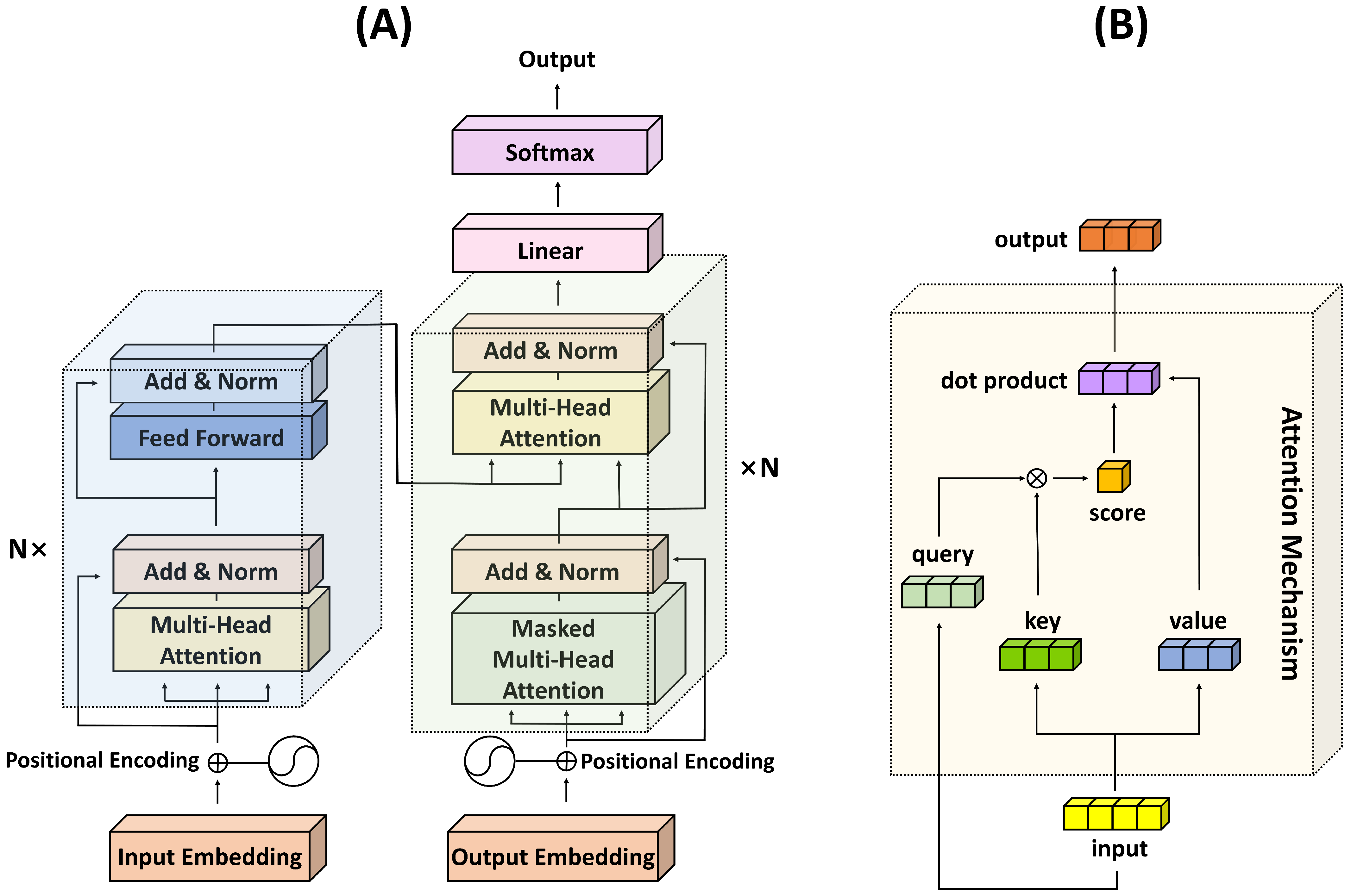
  • Transformers: Have revolutionized natural language processing and are increasingly being used in computer vision. They rely on the "attention mechanism" to weigh the importance of different parts of the input sequence.
  • Autoencoders: Unsupervised learning models that aim to learn a compressed representation of the input data. They consist of an encoder that maps the input to a lower-dimensional latent space and a decoder that reconstructs the original input from the latent representation.
  • Generative Adversarial Networks (GANs): Consist of two neural networks, a generator and a discriminator, that compete with each other. The generator tries to create realistic data samples, while the discriminator tries to distinguish between real and generated data. GANs are powerful for generating new data, such as images, music, and text.

The Deep Learning Workflow

A typical deep learning project involves the following steps:

1. Data Collection and Preprocessing: Gathering relevant data and preparing it for training (e.g., cleaning, normalizing, splitting into training, validation, and test sets).
2. Model Architecture Design: Choosing an appropriate neural network architecture based on the task and data.
3. Training: Feeding the training data to the model and using an optimization algorithm to adjust the weights and biases to minimize the loss function.
4. Validation: Evaluating the model's performance on the validation set during training to tune hyperparameters and prevent overfitting.
5. Testing: Evaluating the final trained model on the unseen test set to get an estimate of its generalization performance.
6. Deployment: Integrating the trained model into a real-world application.

The Future of Deep Learning

Deep learning is a rapidly evolving field with ongoing research and development. Some exciting areas of future exploration include:

• Explainable AI (XAI): Developing methods to make deep learning models more transparent and interpretable.
• Self-Supervised Learning: Training models on unlabeled data by creating artificial labels from the data itself.
• TinyML: Deploying deep learning models on resource-constrained devices like microcontrollers.
• Neuromorphic Computing: Developing new hardware architectures inspired by the human brain.
• Graph Neural Networks (GNNs): Extending deep learning to graph-structured data.
• Reinforcement Learning (RL): Training agents to make optimal decisions in an environment through trial and error, often combined with deep neural networks (Deep RL).

Conclusion

Deep learning has emerged as a powerful paradigm for tackling complex problems across various domains. Its ability to learn intricate patterns from data through multi-layered neural networks has led to significant breakthroughs. While challenges like interpretability and computational cost remain, ongoing research and advancements in algorithms and hardware continue to push the boundaries of what's possible. This comprehensive overview provides a solid foundation for understanding the core concepts and technical intricacies of deep learning, paving the way for further exploration and application of this transformative technology.